 Applied Differential Equations
- Verberg vooruitgang Hide progress Toon vooruitgang Show progress
- Verwijder je antwoorden (op deze pagina) Remove your answers (on this page)
Applied Differential EquationsA first order differential equation that can be written in the form \(\dfrac {dy}{dt}=f(y)\) is autonomous.
Constant functions \(y=C\) such that \(f(C)=0\) satisfy the de on \((-\infty ,\infty )\). These constant solutions are called
equilibrium solutions.
(Note: Same definition applies for \(y'=f(t,y)\). Any constant function \(y=C\) such that \(f(t,C)=0\) is called an
equilibrium solution.)
Here are a few useful properties of first order autonomous differential equations
Example: Let’s consider resource-limited population growth. Let \(p(t)\) represent the size of
a population at time \(t\). When resources are restricted we can employ a \(``\)competition
factor" \(-bp^{2}\), so that \(\displaystyle \frac {dp}{dt}=rp-bp^{2}=rp\left (1-\dfrac {p}{K}\right )\), where \(K=\dfrac {r}{b}\).
This model is called a logistic equation and is a nice example of an autonomous equation. This differential equation has equilibrium solutions at \(p=0\) and \(p=K\). We call \(K\) the \(``\)carrying capacity" of the model and \(r\) the \(``\)intrinsic growth rate."
Let’s determine the \(``\)stability" of these equilibrium values. Assume \(r>0\) and \(K>0\) (negative
values would make no sense for this model).
To do this we plot \(\dfrac {dp}{dt}\) versus \(p\) for \(\dfrac {dp}{dt}=rp\left (1-\dfrac {p}{K}\right )\)
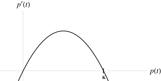
The graph is a parabola with \(x\)-intercepts \((0,0)\) and \((K,0)\).
Note: If \(0<p<K\) then \(\dfrac {dp}{dt}>0\) and \(p\) is increasing. If \(p>K\) then \(\dfrac {dp}{dt}<0\) and \(p\) is decreasing. So if \(p\) is close to \(K\) then \(p\)
is \(``\)pushed" towards \(K\). A similar analysis shows that if \(p\) is close to \(0\) it will be \(``\)pushed"
away from \(0\).
(While we get \(\dfrac {dp}{dt}<0\) when \(p<0\), it’s not relevant to the model as \(p\) cannot be negative.)
We can use arrows to indicate how \(p\) is \(``\)pushed." Here it is with the logistic
equation:
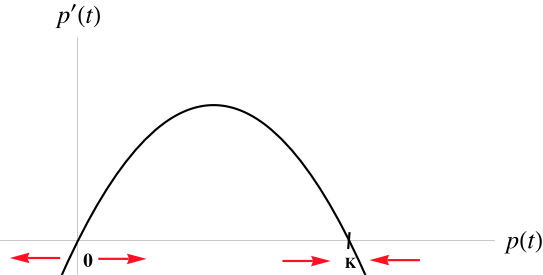
For \(y'=f(y)\), an equilibrium solution \(y=C\) is called an asymptotically stable equilibrium solution
if small perturbations (changes) are \(``\)pushed" back towards \(y=C\). An equilibrium
solution \(y=C\) is called an asymptotically unstable equilibrium solution if small
perturbations will \(``\)push" \(y\) away from \(y=C\). An equilibrium solution \(y=C\) where the
asymptotic behavior depends on which direction the perturbation is called
an
asymptotically semistable equilibrium solution.
With the arrows, just the horizontal axis is called the phase line. Often these are drawn vertically.
Example: Find and classify the equilibrium solutions of \(\dfrac {dy}{dt}=(1-y)(2-y)\).
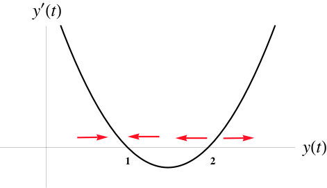
The equilibrium solutions are \(y=1\) and \(y=2\). Since \(y'\) is positive outside of the interval \([1,2]\) and
negative inside \((1,2)\), \(y=1\) is a stable solution and \(y=2\) is an unstable solution.
Another example: Find and classify the equilibrium solutions of \(\dfrac {dy}{dt}=y(2-y)^{2}\).
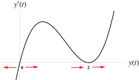
The equilibrium solutions are \(y=0\) and \(y=2\). \(y=0\) is an unstable solution and \(y=2\) is a semistable solution since it is stable from one side (in this case from below) while unstable from the other side (in this case from above).
Yet another example: Find and classify the equilibrium solutions of \(\dfrac {dy}{dt}=\sin {(y)}\).
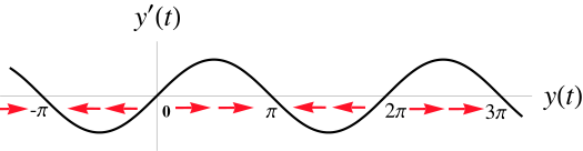
Unstable equilibria exist at \(t=0, \pm 2\pi ,\pm 4\pi ,...\)
Stable equilibria exist at \(t=\pm \pi ,\pm 3\pi ,...\)