There are many applications for first order differential equations.

The classic exponential model \(y'(t)=ky\), \(y(t_{0})=y_{0}\) can be used to model unrestricted population growth \((k>0)\), radioactive decay \((k<0)\), etc.

We have already seen the logistic model \(y'(t)=ry\left (1-\frac {y}{K}\right )\), \(y(t_{0})=y_{0}\) which can model resource-restricted population growth, the spreading of news or a rumor, etc.

Here is a twist on the exponential model:

Suppose that a radioactive substance has decay constant \(k>0\) (reported as a positive number, so use \(y'=-ky\) in the model). At the same time the substance is being produced at a constant rate of \(a\) units of mass per unit time. Let \(y(t)\) be the amount of the substance at time \(t\) and \(y(0)=y_{0}\) be the initial mass.

First we derive a differential equation: \(y'(t)=\mbox { the rate of increase in }y\mbox { }-\mbox { the rate of decrease in }y.\)

So \(y'(t)=a-ky\). Either \(\displaystyle y=\frac {a}{k}\) (equilibrium solution) or \(\displaystyle \frac {1}{a-ky}y'=1\rightarrow \)
\(\displaystyle -\frac {1}{k}\ln {|a-ky|}=t+C\rightarrow \) \(\displaystyle a-ky=\pm e^{-kt+C}\rightarrow \) \(\displaystyle a-ky=Ce^{-kt}\rightarrow \) \(\displaystyle y=\frac {a}{k}+Ce^{-kt}\)
(which includes the constant equilibrium solution if we allow \(C=0\)).

In terms of \(y(0)=y_0\) we get \(\displaystyle y=\frac {a}{k}+\left (y_0-\frac {a}{k}\right )e^{-kt}\). In particular, if \(y_{0}>a/k\) then \(y\) decreases toward the equilibrium solution, and if \(y_{0}<a/k\) then \(y\) increases towards the equilibrium solution.

Another common model is Newton’s Law of Cooling: If an object of temperature \(T(t)\) at time \(t\) is in a medium of temperature \(T_{m}(t)\) at time \(t\) then the rate of change in \(T(t)\) is proportional to the \(\Delta T = T(t)-T_{m}(t)\). When \(T(t)>T_{m}(t)\) we have \(T'(t)<0\) (cooling) and when \(T(t)<T_{m}(t)\) we have \(T'(t)>0\) (warming).

So \(T(t)\) satisfies \(T'=-k(T-T_{m})\) where \(k>0\).

Note: If \(T_m (t)\) is a constant function this model is essentially a shifted exponential decay model.

Mixing applications: Involve the amount \(y\) of something that is mixed, and

\(y'=\) the rate of \(y\) coming in MINUS the rate of \(y\) going out, \(y(0)=\) the initial amount.

Example: A \(500\) L tank initially contains \(2\) kg of salt dissolved in \(100\) L of water. Saltwater that contains \(0.1\) kg of salt per liter is pumped into the tank at \(4\) liters per minute and at the same time water is drained from the tank at \(2\) liters per minute. Assume the tank is always kept uniformly mixed. Calculate the amount of salt in the tank when the tank begins to overflow.

Let \(t\) represent time in minutes (where \(t=0\) corresponds with the initial state of the tank). First note that after \(t\) minutes the volume in the tank is \(V(t)=100+2t\) L so the tank begins to overflow at \(t=200\) (each minute a net gain of 2 L of saltwater goes into the tank and the tank has \(400\) L of space for the incoming saltwater).

Let \(y(t)\) be the amount of salt in kg at time \(0\leq t\leq 200\). At time \(t=0\), \(y(0)=2\).

\(y'(t)=\) rate of salt in \(\;-\;\) rate of salt out \(\displaystyle =\left (\frac {0.1 \;\mathrm {kg}}{\mathrm {L}}\right )\left (\frac {4\; \mathrm {L}}{\mathrm {min} }\right )-\left (\frac {y(t)\; \mathrm {kg}}{100+2t\;\mathrm {L}}\right )\left (\frac {2\;\mathrm {L}}{\mathrm {min}}\right )\).

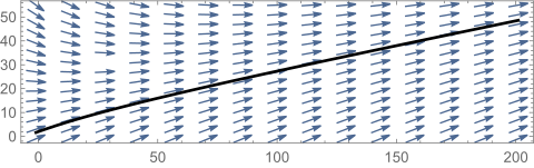
So we have an IVP (simplified): \(\displaystyle y'=\frac {2}{5}-\frac {y}{50+t}\), \(y(0)=2\). While not separable, it is linear:

In standard form, \(\displaystyle y'+\frac {1}{t+50}\,y=\frac {2}{5}\). An integrating factor would be \(\mu (t)=e^{\ln {(t+50)}}=t+50\).

So \(\displaystyle (t+50)\, y'+ y=\frac {2}{5}t+20\rightarrow \) \(\displaystyle \left [(t+50)y\right ]'=\frac {2}{5}t+20\rightarrow \) \(\displaystyle (t+50)y=\frac {1}{5}t^2+20t+C\rightarrow \)

\(\displaystyle y=\frac {\frac {1}{5}t^2+20t+C}{t+50}\). Using \(y(0)=2\) we see that \(C=100\). So \(\displaystyle y=\frac {\frac {1}{5}t^2+20t+100}{t+50}\)

and at the time of overflow, \(\displaystyle y(200)=\frac {\frac {1}{5}(200)^2+20(200)+100}{200+50}=\frac {12,100}{250}=48.4\) kg of salt is in the tank.