 PreCalculus
- Verberg vooruitgang Hide progress Toon vooruitgang Show progress
- Verwijder je antwoorden (op deze pagina) Remove your answers (on this page)
PreCalculusWe begin this section by revisiting (again!) the notion of average velocity - a concept we first encountered in Example ARCRocketExample in Section LinearFunctions and later revisited in Example averagevelocityrocketex in Section IntroRational.
In this scenario, the position function \(s(t) = -5t^2+100t\), \(0 \leq t \leq 20\) gives the height of a model rocket above the Moon’s surface, in feet, \(t\) seconds after liftoff. The average rate of change of \(s\) over an interval is the average velocity of the rocket over that interval. The average velocity provides two pieces of information: the average speed of the rocket along with the rocket’s direction. We formalized the average velocity in Definition averagevelocitydefn in Section IntroRational:
Definition. Let \(s(t)\) be the position of an object at time \(t\) and \(t_{0}\) a fixed time in the domain of \(s\). The average velocity between time \(t\) and time \(t_{0}\) for \(t \neq t_{0}\) is given by
If we define the change in time, \(\Delta t = t - t_{0}\), we get \(t = t_{0} + \Delta t\) which gives:
The above formula measures the average velocity between time \(t_{0}\) and time \(t_{0} + \Delta t\) as a function of \(\Delta t\).
We now revisit Example averagevelocityrocketex in Section IntroRational using this new formulation.
To find \(\overline {v}(\Delta t)\), we first find \(s(15+\Delta t)\):
Since \(s(15) = -5(15)^2 + 100(15) = 375\), we get:
In addition to \(\Delta t \neq 0\), the domain of \(s\) is restricted to \(0 \leq t \leq 20\). Hence, we require \(0 \leq 15 + \Delta t \leq 20\) or \(-15 \leq \Delta t \leq 5\). Our final answer is \(\overline {v}(\Delta t) = -5 \Delta t - 50\), for \(\Delta t \in [-15, 0) \cup (0, 5]\).
Since \(\overline {v}(\Delta t) = -5 \Delta t - 50\), for all values of \(\Delta t\) near \(\Delta t = 0\) (excluding \(\Delta t = 0\)), Theorem limitsagree applies. We get \(\lim _{\Delta t \rightarrow 0} \overline {v}(\Delta t) = \lim _{\Delta t \rightarrow 0} -5 \Delta t - 50 = -5(0) - 50 = -50\), where we have used the fact that the function \(f(\Delta t) = -5 \Delta t - 50\) is continuous to evaluate the limit.
Recall from Example averagevelocityrocketex that the limit value here, \(-50\) is the so-called instantaneous velocity of the rocket at \(t=15\) seconds. That is, \(15\) seconds after lift-off, the rocket is heading back towards the surface of the moon at a rate of \(50\) feet per second.
Since the domain of \(\overline {v}\) is \([-15, 0) \cup (0, 5]\), the graph of \(y = \overline {v}(\Delta t) = -5 \Delta t - 50\) is a line segment from \((-15, 25)\) to \((5, -75)\) with a hole at \((0, -50)\).
![[Picture]](IntroductiontoDerivatives.online-1f9d914e488e4d41d8a9abd8966a915f.svg)
The reader is invited to compare Example averagevelocityrocketex in Section IntroRational with Exercise averagevelocityrocketexreprise above. We obtain the exact same information because we are asking the exact same questions - they are just framed differently. We now take the time to formally define instantaneous velocity:
provided this limit exists.
Based on our work in Examples averagevelocityrocketex and averagevelocityrocketexreprise, we have \(v(15) = -50\). In both of those examples, we’ve seen what \(v(15)\) means on the graph of \(\overline {v}\), but there is a more important interpretation when we analyze the graph of \(s\). Recall that the average velocity, and, more generally, average rates of change can be visualized as slopes of secant lines.
Below is a sequence of secant lines along with the graph of \(y = s(t)\). In each case, the secant line is graphed between \((15, s(15)) = (15, 375)\) and another point on the graph. As the points on the parabola approach \((15, 375)\) the secant lines approach what is known as the tangent line.
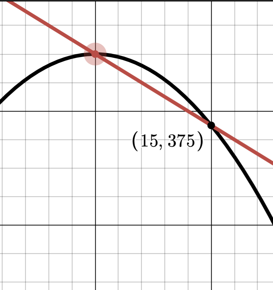 | 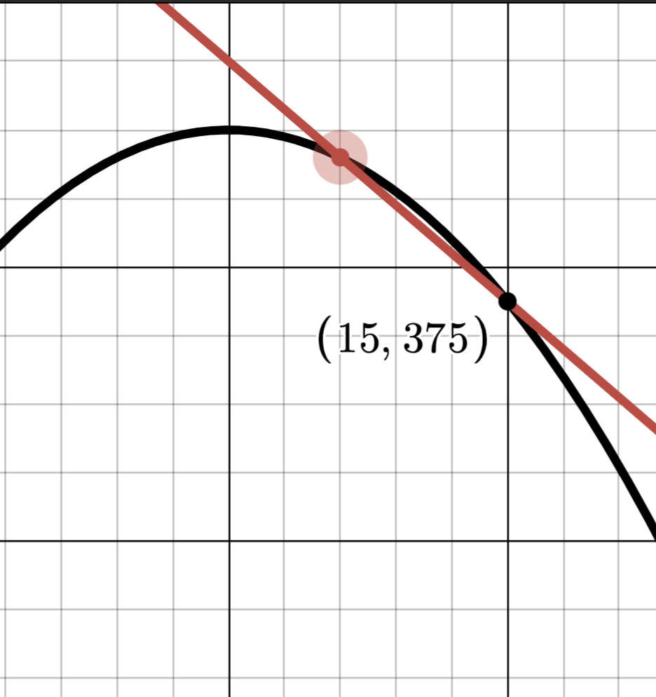 | 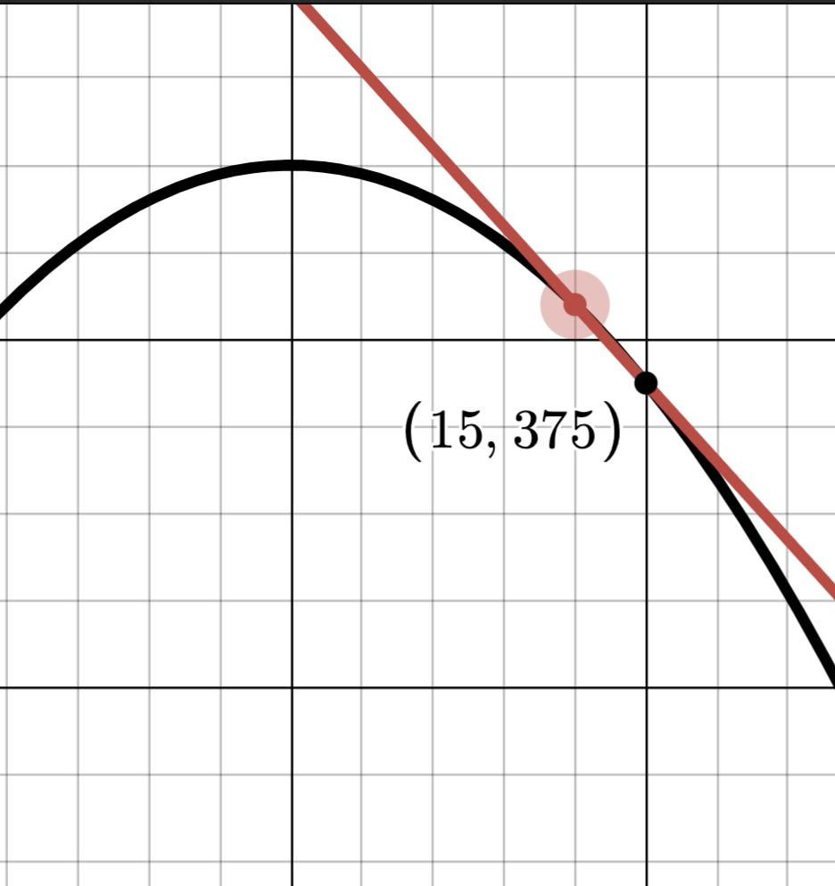 |
To find the equation of the tangent line in this case, which we’ll call \(L(t)\), we refer to the point-slope form of a line, Equation linearfunctionpointslope:
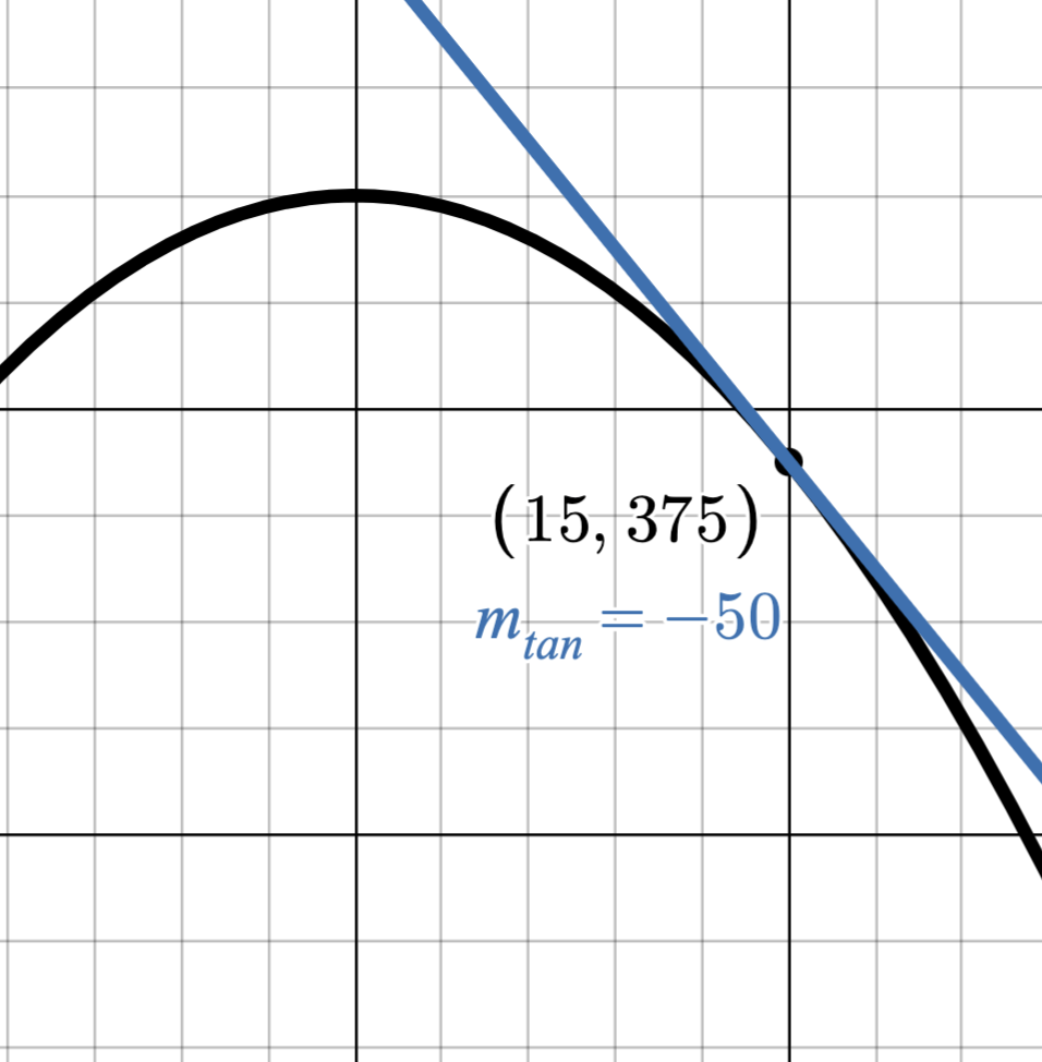
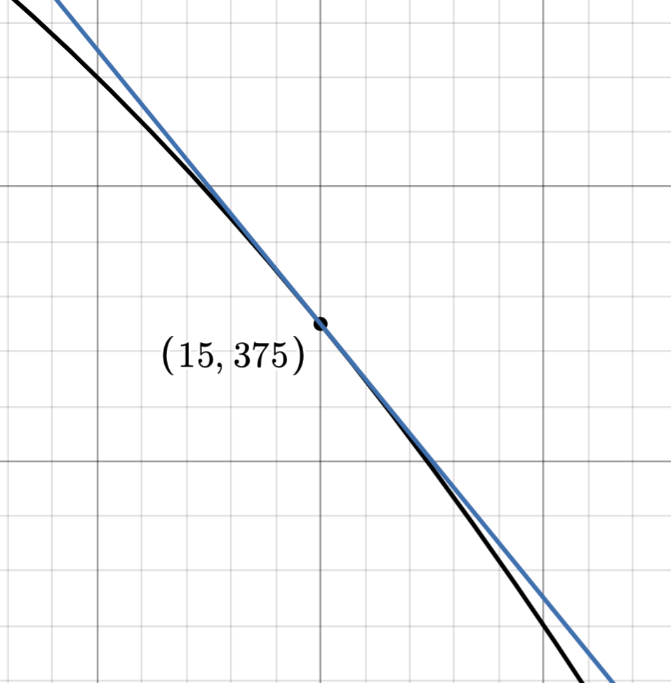
The tangent line can best be thought of as ‘the best linear approximation’ to the graph of \(y = s(t)\) at \((15,375)\). That is, if we zoom in near \((15,375)\), the graph of \(y = s(t)\) and this tangent line become indistinguishable. This geometric property of \(y = s(t)\) is called local linearity and is foundational to the analysis of functions. Below we graph \(y = s(t) = -5t^2+100t\) along with \(y = L(t) = -50t + 1125\) and observe the local linearity near \((15, 375)\).
 |
 |
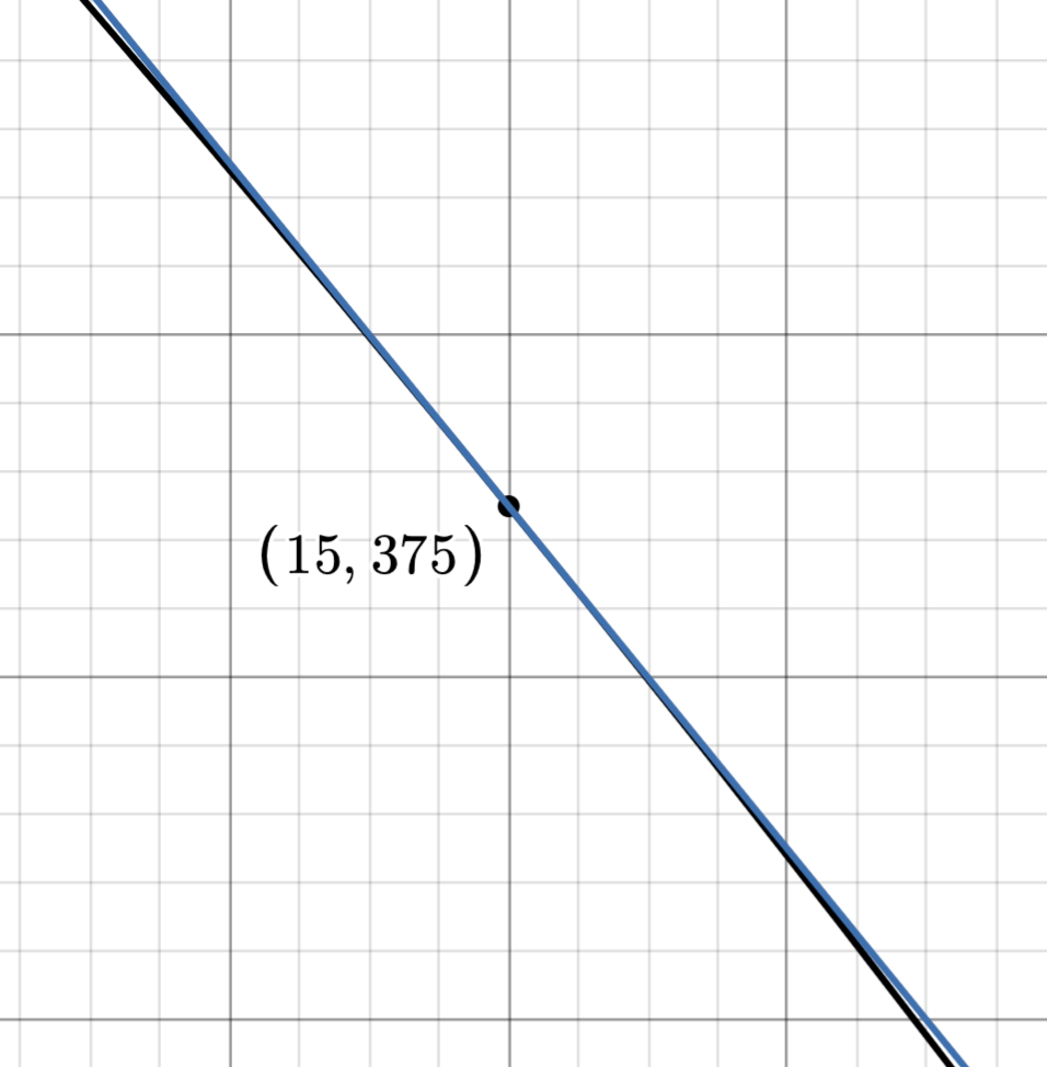 |
| The tangent line at \((15, 375)\). | Zooming in near \((15, 375)\). | Zooming in closer to \((15, 375)\). |
Using desmos, we can more smoothly visualize this process using the interactive below. By dragging the highlighted point along the graph of \(y=s(t)\) closer to \((15, 375)\), we can observe the secant lines approaching the tangent line.
Our next step is to generalize these notions to all functions.
Recall in Section AverageRateofChange the concept of the average rate of change of a function over the interval \([a,b]\) is the slope between the two points \((a, f(a))\) and \((b, f(b))\) and is given by
Geometrically, the average rate of change is the slope of the so-called secant line which ‘cuts’ through the graph of \(y = f(x)\) at the points \((a,f(a))\) and \((b, f(b))\):
![[Picture]](IntroductiontoDerivatives.online-9e726f0e604bfb49f6169bd75524a284.svg)
Consider a function \(f\) defined over an interval containing \(x\) and \(x+h\) where \(h \neq 0\). The average rate of change of \(f\) over the interval \([x,x+h]\) is thus given by the formula:
The above is an example of what is traditionally called the difference quotient or Newton quotient of \(f\), since it is the quotient of two differences, namely \(\Delta [f(x)]\) and \(\Delta x\). Another formula for the difference quotient (as seen in Section rocarithmetic) keeps with the notation \(\Delta x\) instead of \(h\):
It is important to understand that in this formulation of the difference quotient, the variables ‘\(x\)’ and ‘\(\Delta x\)’ are distinct - that is they do not combine as like terms.
Note that, regardless of which form the difference quotient takes, when \(h\), \(\Delta x\), or \(\Delta t\) is \(0\), the difference quotient returns the indeterminate form ‘\(\frac {0}{0}\).’ As we’ve seen with rational functions in Section IntroRational, when this happens, we can use a limit to help us determine the indeterminate form.
In Section avginstantvelocity, taking the limit of average velocity as \(\Delta t \rightarrow 0\) produced instantaneous velocity. More generally, taking the limit of the average rate of change as the denominator approaches \(0\) produces the instantaneous rate of change of the function at that point. The instantaneous rate of change of a function, called the derivative of the function, is defined below.
The number \(f'(a)\) represents the instantaneous rate of change of \(f\) with respect to \(x\) at the input \(x = a\). If \(f'(a)\) exists, we say \(f\) is differentiable at \(x = a\).
Using the language of derivatives, Examples averagevelocityrocketex and averagevelocityrocketexreprise have us computing \(v(15) = s'(15)\). Moreover, since the derivative is a rate of change, it’s important to note that the associated units of \(f'(a)\) are \(\frac { \text {units of $f(x)$}}{\text {units of $x$}}\). This tracks with the units of \(v(15) = s'(15)\) being \(\frac { \text {feet}}{\text {second}}\), a velocity.
As in Section avginstantvelocity, \(f'(a)\) represents the slope of the tangent line at the point \((a, f(a))\). We use this to formally define the tangent line below.
We put these definitions to good use in the following example.
We first find \(m_{\text {tan}} = f'(-2)\) using Definition derivativedefn with \(a = -2\): \( f'(-2) = \lim _{h \rightarrow 0} \frac {f(-2+h) - f(-2)}{h}\).
First we find \(f(-2+h)\) and are careful to apply the exponent in the expression \(-(-2+h)^2\):
Next, we find \(f(-2) = -(-2)^2 + 3(-2)-1 = -11\), so the difference quotient is:
Finally, we get \( f'(-2) = \lim _{h \rightarrow 0} \frac {f(-2+h) - f(-2)}{h} = \lim _{h \rightarrow 0} (-h+7) = -(0) + 7 = 7\).
Hence, the slope of the tangent line is \(m_{\text {tan}} = f'(-2) = 7\). The equation of the tangent line is:
Graphing \(y = 7x+3\) and \(y = f(x)\) near \((-2,-11)\) reveals the local linearity we would expect. Using the desmos graph below, we can zoom in on the point \((-2,-11)\) to our heart’s content until the graph of \(y = f(x)\) and the tangent line become indistinguishable.
What if we wanted to find the equation of the tangent line to the graph of the function in Example tangentlineex at \(x = 0\)? \(x = 1\)? \(x = 5\)? We’d ostensibly need to run through difference quotients and limit calculations for each and every input value: \(x = 0\), \(x = 1\), and \(x = 5\). Or we could do a single limit with a generic ‘\(x\)’, simplify the difference quotient and take the limit once, and substitute in particular values of \(x\):
provided the limit exists.
It is worth noting that if we set \(h = \Delta x\), and consider the graph \(y = f(x)\), we get:
which is why sometimes the derivative is denoted \(\frac {dy}{dx}\).
To find \(f'(x) = \lim _{h \rightarrow 0} \frac {f(x+h) - f(x)}{h}\) we first find \(f(x+h)\):
The difference quotient simplifies as follows:
Our last step is to take the limit: \(f'(x) = \lim _{h \rightarrow 0} \frac {f(x+h) - f(x)}{h} = \lim _{h \rightarrow 0} (-2x-h+3)\). Notice here that we have two variables, \(x\) and \(h\), in the limit. Of these two variables, we are taking the limit on the \(h\): \(h \rightarrow 0\). As far as \(h\) is concerned, \(x\) may as well be just another constant like the ‘\(3\)’. Hence, \(f'(x) = \lim _{h \rightarrow 0} (-2x-h+3)= -2x - 0 + 3 = -2x+3\).
The equation of the tangent line to the graph of \(y = f(x)\) at \(x = 0\) is \(y = f'(0) (x - 0) + f(0)\). We have \(f'(0)=2(0) + 3 = 3\) and \(f(0) = -(0)^2+3(0)-1 = -1\). We get \(y = 3(x-0)+(-1)\) so \(y = 3x-1\). Our graph bears this out.
Solving \(f'(x) = 0\) gives \(-2x+3 = 0\) so \(x = \frac {3}{2}\). This means the slope of the tangent line at the point \(\left (\frac {3}{2}, f\left (\frac {3}{2}\right ) \right )\) is \(0\), so the tangent line there is horizontal. We find \(f\left (\frac {3}{2}\right ) = -\left ( \frac {3}{2}\right )^2 + 3\left (\frac {3}{2}\right ) - 1 = \ldots = \frac {5}{4}\). Hence, the tangent line at \(\left (\frac {3}{2}, \frac {5}{4} \right )\) is \(y = \frac {5}{4}\). Graphically, this checks out.
The astute reader will note that the graph of \(f(x) = -x^2+3x-1\) in Example derivativeex is a parabola and finding where \(f'(x) = 0\) lead us right back to the vertex. Using a derivative to find the vertex may seem a bit excessive given that we’ve algebraically derived a handy ‘vertex formula’ in Section QuadraticFunctions. However, as the functions we aim to analyze become more and more sophisticated, the tools we use to analyze them must also become more sophisticated. The derivative is one such tool that has a near universal application.
For \(f(x) = x^2-x-2\), find and simplify:
The equation of the tangent line to the graph \(y = f(x)\) at \((3, f(3))\).
Check your answer graphically.
For \(g(x) = \frac {3}{2x+1}\), find and simplify:
The equation of the tangent line to the graph \(y = g(x)\) at \((0, g(0))\).
Check your answer graphically.
\(r(t) = \sqrt {t}\), find and simplify:
The equation of the tangent line to the graph \(y = r(t)\) at \((9, r(9))\).
Check your answer graphically.
To find \(f'(3) =\lim _{h \rightarrow 0}\) \(\frac {f(3+h)-f(3)}{h}\) we first simplify \(f(3+h)\):
Since \(f(3) = (3)^2-3-2 = 4\), we get for the difference quotient:
The equation of the tangent line at \(x = 3\) is: \(y = f'(3)(x-3) + f(3) = 5(x-3) + 4\), or \(y = 5x-11\). We check graphically below.
To find \(f'(x) = \lim _{h \rightarrow 0}\frac {f(x+h)-f(x)}{h}\), we first find \(f(x+h)\):
So the difference quotient is
Hence, \(f'(x) = \lim _{h \rightarrow 0} (2x+h-1) = 2x + 0 - 1\) so \(f'(x) = 2x-1\). Note that using this formula, we get \(f'(3) = 2(3)-1 = 5\) which checks our answer above.
Next we find \(g'(0) = \lim _{h \rightarrow 0} \frac {g(0+h)-g(0)}{h} = \frac {g(h) - g(0)}{h}\).
Since \(g(h) = \frac {3}{2 h + 1}\) and \(g(0) = \frac {3}{2(0)+1} = 3\), our difference quotient contains a complex fraction. Thinking ahead, we need to (eventually) be able to cancel the factor ‘\(h\)’ from the denominator \(\frac {g(h) - g(0)}{h}\), so we begin by simplifying the complex fraction and see where that takes us:
We are now ready to take the limit:
The equation of the tangent line when \(x = 0\) is: \(y = g'(0)(x-0) + g(0) = (-6)(x-0)+ 3\) or \(y = -6x+3\), which checks graphically below.
To find \(g'(x)\), we first find \(g(x+h)\):
Simplifying the difference quotient involves simplifying the resulting complex fraction, as above, keeping an eye out for an opportunity to cancel the factor ‘\(h\)’ from the denominator:
Hence,
To find \(r'(9) = \lim _{h \rightarrow 0}\frac {r(9+h) - r(9)}{h}\), we start with \(r(9+h) = \sqrt {9+h}\) and \(r(9) = \sqrt {9} = 3\). Hence our difference quotient is:
In order for us to determine the limit as \(h \rightarrow 0\), we need to somehow cancel the factor of \(h\) from the denominator. To do so, we set about rationalizing the numerator by multiplying both numerator and denominator by the conjugate of the numerator, \(\sqrt {9+h} - 3\):
Hence,
The equation of the tangent line to \(y = r(t)\) at \((9,3)\) is therefore: \(y = r'(9)(t-9) + r(9) = \frac {1}{6} (t-9) + 3\) or \(y = \frac {1}{6} \, t + \frac {3}{2}\). The graph below confirms this.
As one might expect, we use this same strategy of rationalizing the numerator to simplify the difference quotient to find \(r'(t)\):
We get