Je bent je ingevulde velden bij deze pagina aan het verwijderen. Ben je zeker dat je dit wilt doen?
You are erasing your filled-in fields on this page. Are you sure that is what you want?
Nieuwe Versie BeschikbaarNew Version Available
Er is een update van deze pagina. Als je update naar de meest recente versie, verlies je mogelijk je huidige antwoorden voor deze pagina. Hoe wil je verdergaan ?
There is an updated version of this page. If you update to the most recent version, then your current progress on this page will be erased. Regardless, your record of completion will remain. How would you like to proceed?
In Exercises paraplotfirst - paraplotlast, plot the set of parametric equations by hand. Be sure to indicate the orientation imparted on the curve by
the parametrization.
\( \left \{ \begin{array}{l} x = 4t-3 \\ y = 6t-2 \end{array} \right . \text {for } 0 \leq t \leq 1\)
\( \left \{ \begin{array}{l} x = 4t-1 \\ y = 3-4t \end{array} \right . \text {for } 0 \leq t \leq 1\)
\( \left \{ \begin{array}{l} x = 2t \\ y = t^2 \end{array} \right . \text {for } -1 \leq t \leq 2\)
\( \left \{ \begin{array}{l} x = t-1 \\ y = 3+2t-t^2 \end{array} \right . \text {for } 0 \leq t \leq 3\)
\( \left \{ \begin{array}{l} x = t^2+2t+1 \\[3pt] y = t+1 \end{array} \right . \text {for } t \leq 1\)
\( \left \{ \begin{array}{l} x = \frac {1}{9}\left (18-t^2\right ) \\[3pt] y = \frac {1}{3} t \end{array} \right . \text {for } t \geq -3\)
\( \left \{ \begin{array}{l} x = t \\ y = t^3 \end{array} \right . \text {for } -\infty < t < \infty \)
\( \left \{ \begin{array}{l} x = t^3 \\ y = t \end{array} \right . \text {for } -\infty < t < \infty \)
\( \left \{ \begin{array}{l} x = \cos (t) \\ y = \sin (t) \end{array} \right . \text {for } -\frac {\pi }{2} \leq t \leq \frac {\pi }{2}\)
\( \left \{ \begin{array}{l} x = 3\cos (t) \\ y = 3\sin (t) \end{array} \right . \text {for } 0 \leq t \leq \pi \)
\( \left \{ \begin{array}{l} x = -1+ 3\cos (t) \\ y = 4\sin (t) \end{array} \right . \text {for } 0 \leq t \leq 2\pi \)
\( \left \{ \begin{array}{l} x = 3\cos (t) \\ y = 2\sin (t)+1 \end{array} \right . \text {for } \frac {\pi }{2} \leq t \leq 2\pi \)
\( \left \{ \begin{array}{l} x = 2\cos (t) \\ y = \sec (t) \end{array} \right . \text {for } 0 \leq t < \frac {\pi }{2}\)
\( \left \{ \begin{array}{l} x = 2\tan (t) \\ y = \cot (t) \end{array} \right . \text {for } 0 < t < \frac {\pi }{2}\)
\( \left \{ \begin{array}{l} x = \sec (t) \\ y = \tan (t) \end{array} \right . \text {for } -\frac {\pi }{2} < t < \frac {\pi }{2}\)
\( \left \{ \begin{array}{l} x = \sec (t) \\ y = \tan (t) \end{array} \right . \text {for } \frac {\pi }{2} < t < \frac {3\pi }{2}\)
\( \left \{ \begin{array}{l} x = \tan (t) \\ y = 2\sec (t) \end{array} \right . \text {for } -\frac {\pi }{2} < t < \frac {\pi }{2}\)
\( \left \{ \begin{array}{l} x = \tan (t) \\ y = 2\sec (t) \end{array} \right . \text {for } \frac {\pi }{2} < t < \frac {3\pi }{2}\)
\( \left \{ \begin{array}{l} x = \cos (t) \\ y = t \end{array} \right . \text {for } 0 \leq t \leq \pi \)
\( \left \{ \begin{array}{l} x = \sin (t) \\ y = t \end{array} \right . \text {for } -\frac {\pi }{2} \leq t \leq \frac {\pi }{2}\)
In the same way (and for the same reason) we took the time on page ?? in Section PolarGraphs to show how to graph
polar equations using a graphing calculator, we take a few moments here to explain how to graph a system of
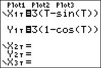
parametric equations using a calculator. Our task is to graph the cycloid from Example cycloidex, \(\left \{ x = 3(t -\sin (t)), \, y = 3(1-\cos (t)) \right .\) for \(t \geq 0\) using a graphing
calculator.
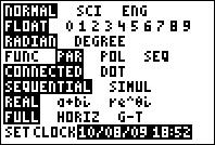
We first must ensure that the calculator is in ‘Parametric Mode’ and ‘radian mode’ when we enter the equations and advance
to the ‘Window’ screen.
Our next step is to find appropriate bounds on the parameter, \(t\), as well as for \(x\) and \(y\). We know that one full revolution of the
circle occurs over the interval \(0 \leq t < 2\pi \), so it seems reasonable to keep these as our bounds on \(t\). The ‘Tstep’ seems reasonably small
– too large a value here can lead to incorrect graphs. (Again, see page ?? in Section PolarGraphs.) We know from our derivation of
the equations of the cycloid that the center of the generating circle has coordinates \((r\theta ,r) = (3t,3)\). Since \(t\) ranges between \(0\) and \(2\pi \), we set \(x\)
to range between \(0\) and \(6\pi \). The values of \(y\) go from the bottom of the circle to the top, so \(y\) ranges between \(0\) and
\(6\).
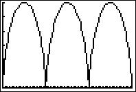
Below we graph the cycloid with these settings, and then extend \(t\) to range from \(0\) to \(6\pi \) which forces \(x\) to range from \(0\) to \(18\pi \) yielding
three arches of the cycloid. (It is instructive to note that keeping the \(y\) settings between 0 and 6 skews the aspect ratio of
the cycloid. Using the ‘Zoom Square’ feature on the graphing calculator gives a true geometric perspective of the three
arches.)
In Exercises paracalcfirst - paracalclast, plot the set of parametric equations with the help of a graphing utility. Be sure to indicate the orientation
imparted on the curve by the parametrization.
\( \left \{ \begin{array}{l} x = t^{3} - 3t \\ y = t^{2} - 4 \end{array} \right . \text {for } -2 \leq t \leq 2\)
\( \left \{ \begin{array}{l} x = 4\cos ^{3}(t) \\ y = 4\sin ^{3}(t) \end{array} \right . \text {for } 0 \leq t \leq 2\pi \)
\( \left \{ \begin{array}{l} x = e^{t} + e^{-t} \\ y = e^{t} - e^{-t} \end{array} \right . \text {for } -2 \leq t \leq 2\)
\( \left \{ \begin{array}{l} x = \cos (3t) \\ y = \sin (4t) \end{array} \right . \text {for } 0 \leq t \leq 2\pi \)
Use parametric equations and a graphing utility to graph the inverse of \(f(x) = x^{3} + 3x - 4\).
The parametric equations for the inverse are \( \left \{ \begin{array}{l} x = t^3+3t-4 \\ y = t \end{array} \right . \text {for } -\infty < t < \infty \)
Every polar curve \(r = f(\theta )\) can be translated to a system of parametric equations with parameter \(\theta \) by \(\left \{ x = r\cos (\theta ) = f(\theta ) \cos (\theta ), \, y = r \sin (\theta ) = f(\theta ) \sin (\theta ) \right .\). Convert \(r = 6\cos (2\theta )\) to a system of
parametric equations. Check your answer by graphing \(r = 6\cos (2\theta )\) by hand using the techniques presented in Section PolarGraphs and then graphing
the parametric equations you found using a graphing utility.
Suppose an object, called a projectile, is launched into the air. Ignoring everything except the force gravity, the path of the
projectile is given by (A nice mix of vectors and Calculus are needed to derive this.)
\[ \left \{ \begin{array}{l} x = v_{0} \cos (\theta ) \, t \\ y = -\frac {1}{2} g t^2 + v_{0} \sin (\theta ) \, t + s_{0} \\ \end{array} \right . \; \text {for } \; 0 \leq t \leq T \]
where \(v_{0}\) is the initial speed of the object, \(\theta \) is the angle from the horizontal at which the projectile is launched, (We’ve seen
this before. It’s the angle of elevation which was defined on page ??.)\(g\) is the acceleration due to gravity, \(s_{0}\) is the initial
height of the projectile above the ground and \(T\) is the time when the object returns to the ground. (See the figure
below.)
Carl’s friend Jason competes in Highland Games Competitions across the country. In one event, the ‘hammer throw’, he
throws a 56 pound weight for distance. If the weight is released \(6\) feet above the ground at an angle of \(42^{\circ }\) with respect to the
horizontal with an initial speed of \(33\) feet per second, find the parametric equations for the flight of the hammer. (Here, use \(g = 32 \frac {\text {ft.}}{s^2}\).)
When will the hammer hit the ground? How far away will it hit the ground? Check your answer using a graphing
utility.
The parametric equations for the hammer throw are \( \left \{ \begin{array}{l} x = 33 \cos (42^{\circ }) t \\ [4pt] y =-16t^2 + 33 \sin (42^{\circ }) t + 6 \end{array} \right .\) for \(t \geq 0\).
To find when the hammer hits the ground, we solve \(y(t) = 0\) and get \(t \approx -0.23\) or \(1.61\). Since \(t \geq 0\), the hammer hits the ground after approximately \(t = 1.61\)
seconds after it was launched into the air.
To find how far away the hammer hits the ground, we find \(x(1.61) \approx 39.48\) feet from where it was thrown into the air.
Eliminate the parameter in the equations for projectile motion to show that the path of the projectile follows the curve
In another event, the ‘sheaf toss’, Jason throws a 20 pound weight for height. If the weight is released 5 feet above
the ground at an angle of \(85^{\circ }\) with respect to the horizontal and the sheaf reaches a maximum height of 31.5
feet, use your results from part projectileeliminate to determine how fast the sheaf was launched into the air. (Once again, use
\(g = 32 \frac {\text {ft.}}{s^2}\).)
We solve \(y = \frac {v_{0}^2 \sin ^{2}(\theta )}{2g} + s_{0} = \frac {v_{0}^2 \sin ^{2}(85^{\circ })}{2(32)} + 5 = 31.5\) to get \(v_{0} = \pm 41.34\).
The initial speed of the sheaf was approximately \(41.34\) feet per second.
Suppose \(\theta = \frac {\pi }{2}\). (The projectile was launched vertically.) Simplify the general parametric formula given for \(y(t)\) above using \(g = 9.8 \, \frac {m}{s^2}\) and
compare that to the formula for \(s(t)\) given in Exercise whatgoesup in Section QuadraticFunctions. What is \(x(t)\) in this case?
If \(f\) and \(g\) are functions, explain why the function \(\vec {r}(t) = \left <f(t), g(t) \right >\) is a function. The function \(\vec {r}\) is called a vector-valued function since it
matches real number inputs, \(t\), with vector outputs, \(\vec {r}(t)\). Explain why when the vectors \(\vec {r}(t)\) are plotted in standard position, their
terminal points trace out the curve described parametrically by the system of equations: \(\left \{ x = f(t) \, y = g(t) \right .\) (In Calculus, you will see systems of
parametric equations ‘packaged’ together using vectors.)
In Exercises hyperbolicfirst - hyperboliclast, we explore the hyperbolic cosine function, denoted \(\cosh (t)\), and the hyperbolic sine function, denoted \(\sinh (t)\), defined
below:
Using a graphing utility as needed, verify the following:
the domain of \(\cosh (t)\) is \((-\infty , \infty )\) and the range of \(\cosh (t)\) is \([1,\infty )\).
the domain and range of \(\sinh (t)\) are both \((-\infty , \infty )\).
Show that \(\left \{ x(t) = \cosh (t), \, y(t) = \sinh (t) \right .\) parametrize the right half of the ‘unit’ hyperbola \(x^2 - y^2 = 1\). (Hence the use of the adjective ‘hyperbolic.’)
Compare and contrast the definitions of \(\cosh (t)\) and \(\sinh (t)\) to the formulas for \(\cos (t)\) and \(\sin (t)\) given in Exercise expformcosandsin in Section PolarComplex.
Four other hyperbolic functions are waiting to be defined: the hyperbolic secant \(\text {sech}(t)\), the hyperbolic cosecant \(\text {csch}(t)\), the hyperbolic
tangent \(\tanh (t)\) and the hyperbolic cotangent \(\coth (t)\). Define these functions in terms of \(\cosh (t)\) and \(\sinh (t)\), then convert them to formulas involving \(e^{t}\) and \(e^{-t}\).
Consult a suitable reference (a Calculus book, or this entry on the hyperbolic functions) and spend some time reliving the
thrills of trigonometry with these ‘hyperbolic’ functions.

![[Picture]](ExercisesforParametricEquations.online-a65750e7699fac477fe71003e48aa12e.svg)
![[Picture]](ExercisesforParametricEquations.online-5d15b8c5fd6ec6a57624b82d0dea6079.svg)
![[Picture]](ExercisesforParametricEquations.online-e678061abae9a35194482d9b5908160e.svg)
![[Picture]](ExercisesforParametricEquations.online-6f84b4f34a9a9bf71933acdc967f776f.svg)
![[Picture]](ExercisesforParametricEquations.online-11dbba8f31642d67b35e651232445961.svg)
![[Picture]](ExercisesforParametricEquations.online-61e8b71467c9640a15e7a2417e089830.svg)
![[Picture]](ExercisesforParametricEquations.online-7d393e5b7d3bf115f22b393e3f6ff857.svg)
![[Picture]](ExercisesforParametricEquations.online-8ba8ea2629a527956a921f10d652a3fb.svg)
![[Picture]](ExercisesforParametricEquations.online-2ae33c3e46d1106fe83bcd08c73694e3.svg)
![[Picture]](ExercisesforParametricEquations.online-d0537d21b48c6867ebb3f20779d4a917.svg)
![[Picture]](ExercisesforParametricEquations.online-e3f40c62e9e1608158fc7bf030eda4a1.svg)
![[Picture]](ExercisesforParametricEquations.online-1bb55be6dbef56f465b16fddc9d999e4.svg)
![[Picture]](ExercisesforParametricEquations.online-6cd3cd2bd36debf6a43502912f797425.svg)
![[Picture]](ExercisesforParametricEquations.online-3bf21afc65f56ee5fd381f3d76f1ac27.svg)
![[Picture]](ExercisesforParametricEquations.online-4764be8f5dd04b28dd1778e236929248.svg)
![[Picture]](ExercisesforParametricEquations.online-6f37f65e33d8b7d72a9a0e1ec8ddf97f.svg)
![[Picture]](ExercisesforParametricEquations.online-1dcd095c54a151cc16664df9878b1b64.svg)
![[Picture]](ExercisesforParametricEquations.online-6b914b93517e0b6ea24486a4f89463e0.svg)
![[Picture]](ExercisesforParametricEquations.online-4535959fedfd39eb6cefc4f7294c9e47.svg)
![[Picture]](ExercisesforParametricEquations.online-017fcb3b9653b0f39d7b4767f2798dc4.svg)


![[Picture]](ExercisesforParametricEquations.online-3582d62b2089f72de6ce861bc2488642.svg)
![[Picture]](ExercisesforParametricEquations.online-bd0d0781deb2f44830880a095cb285c7.svg)
![[Picture]](ExercisesforParametricEquations.online-fb1f80ed82a33a9d06ec1057331a3de5.svg)
![[Picture]](ExercisesforParametricEquations.online-4dad080a720d656d03f7ab426e46fe1b.svg)
![[Picture]](ExercisesforParametricEquations.online-d3e2c493074bd326a4e9c8b2df3712bf.svg)