Je bent je ingevulde velden bij deze pagina aan het verwijderen. Ben je zeker dat je dit wilt doen?
You are erasing your filled-in fields on this page. Are you sure that is what you want?
Nieuwe Versie BeschikbaarNew Version Available
Er is een update van deze pagina. Als je update naar de meest recente versie, verlies je mogelijk je huidige antwoorden voor deze pagina. Hoe wil je verdergaan ?
There is an updated version of this page. If you update to the most recent version, then your current progress on this page will be erased. Regardless, your record of completion will remain. How would you like to proceed?
Starting with the graph of \(f(x) = x^3\), use Theorem linearmononialgraphs to sketch the graph of \(F(x) = (x + 2)^{3} + 1\). Track at least three points of your choice through the
transformations. State the domain and range of \(F\).
Use the Desmos graph below with the settings \(f(x)=x^3,\,h=-2,\,k=1,\,a=1\)
domain: \((-\infty , \infty )\)
range: \((-\infty , \infty )\)
Starting with the graph of \(f(x) = x^4\), use Theorem linearmononialgraphs to sketch the graph of \(F(x) = (x + 2)^{4} + 1\). Track at least three points of your choice through the
transformations. State the domain and range of \(F\).
Use the Desmos graph below with the settings \(f(x)=x^4,\,h=-2,\,k=1,\,a=1\)
domain: \((-\infty , \infty )\)
range: \([1, \infty )\)
Starting with the graph of \(f(x) = x^4\), use Theorem linearmononialgraphs to sketch the graph of \(F(x) = 2 - 3(x - 1)^{4}\). Track at least three points of your choice through the
transformations. State the domain and range of \(F\).
Use the Desmos graph below with the settings \(f(x)=x^4,\,h=1,\,k=2,\,a=-3\)
domain: \((-\infty , \infty )\)
range: \((-\infty , 2]\)
Starting with the graph of \(f(x) = x^5\), use Theorem linearmononialgraphs to sketch the graph of \(F(x) = -x^5 - 3\). Track at least three points of your choice through the
transformations. State the domain and range of \(F\).
Use the Desmos graph below with the settings \(f(x)=x^5,\,h=0,\,k=-3,\,a=-1\)
domain: \((-\infty , \infty )\)
range: \((-\infty , \infty )\)
Starting with the graph of \(f(x) = x^5\), use Theorem linearmononialgraphs to sketch the graph of \(F(x) = (x + 1)^{5} + 10\). Track at least three points of your choice through the
transformations. State the domain and range of \(F\).
Use the Desmos graph below with the settings \(f(x)=x^5,\,h=-1,\,k=10,\,a=1\)
domain: \((-\infty , \infty )\)
range: \((-\infty , \infty )\)
Starting with the graph of \(f(x) = x^6\), use Theorem linearmononialgraphs to sketch the graph of \(F(x) = 8 - x^6\). Track at least three points of your choice through the
transformations. State the domain and range of \(F\).
Use the Desmos graph below with the settings \(f(x)=x^6,\,h=0,\,k=8,\,a=-1\)
domain: \((-\infty , \infty )\)
range: \((-\infty , 8]\)
Find a formula for the function below in the form \(F(x) = a(x-h)^3+k\).
\(F(x) = \answer {(x-1)^3-2}\)
Find a formula for the function below in the form \(F(x) = a(x-h)^3+k\).
\(F(x) = -\frac {1}{2} (x+2)^3+3\)
Find a formula for the function below in the form \(F(x) = a(x-h)^4+k\).
\(F(x) = 2(x+1)^4-4\)
Find a formula for the function below in the form \(F(x) = a(x-h)^4+k\).
\(F(x) = -0.15625x^4+2.5\)
Find the degree, the leading term, the leading coefficient, the constant term and the end behavior of the polynomial function
\(f(x) = 4-x-3x^2\).
Find the degree, the leading term, the leading coefficient, the constant term and the end behavior of the polynomial function
\(g(x) = 3x^5 - 2x^2 + x + 1\).
Find the degree, the leading term, the leading coefficient, the constant term and the end behavior of the polynomial function
\(f(x) = \sqrt {3}x^{17} + 22.5x^{10} - \pi x^{7} + \frac {1}{3}\).
Find the degree, the leading term, the leading coefficient, the constant term and the end behavior of the polynomial function
\(s(t) = -4.9t^{2} + v_0t + s_0\).
Find the degree, the leading term, the leading coefficient, the constant term and the end behavior of the polynomial function
\(P(x) = (x - 1)(x - 2)(x - 3)(x - 4)\).
Find the degree, the leading term, the leading coefficient, the constant term and the end behavior of the polynomial function
\(p(t) = -t^2(3 - 5t)(t^{2} + t + 4)\).
Find the degree, the leading term, the leading coefficient, the constant term and the end behavior of the polynomial function
\(f(x) = -2x^3(x+1)(x+2)^2\).
Find the degree, the leading term, the leading coefficient, the constant term and the end behavior of the polynomial function \(G(t) = 4(t-2)^2\left (t+\frac {1}{2}\right )\)
.
Find the real zeros of the polynomial \(a(x) = x(x + 2)^{2}\) and their corresponding multiplicities. Use this information along with end behavior to
provide a rough sketch of the graph of the polynomial function. Compare your answer with the result from a graphing
utility.
\(x = 0\) \(\text { multiplicity } {1}\)
\(x = -2\) \(\text { multiplicity } {2}\)
Find the real zeros of the polynomial \(g(t) = t(t + 2)^{3}\) and their corresponding multiplicities. Use this information along with end behavior to
provide a rough sketch of the graph of the polynomial function. Compare your answer with the result from a graphing
utility.
\(t = 0\) \(\text { multiplicity } {1}\)
\(t = -2\) \(\text { multiplicity } {3}\)
Find the real zeros of the polynomial \(f(z) = -2(z-2)^2(z+1)\) and their corresponding multiplicities. Use this information along with end behavior to
provide a rough sketch of the graph of the polynomial function. Compare your answer with the result from a graphing
utility.
\(z = 2\) \(\text { multiplicity } {2}\)
\(z = -1\) \(\text { multiplicity } {1}\)
Find the real zeros of the polynomial \(g(x) = (2x+1)^2(x-3)\) and their corresponding multiplicities. Use this information along with end behavior to
provide a rough sketch of the graph of the polynomial function. Compare your answer with the result from a graphing
utility.
Find the real zeros of the polynomial \(F(t) = t^{3}(t+ 2)^{2}\) and their corresponding multiplicities. Use this information along with end behavior to
provide a rough sketch of the graph of the polynomial function. Compare your answer with the result from a graphing
utility.
\(t = 0\) \(\text { multiplicity } {3}\)
\(t = -2\) \(\text { multiplicity } {2}\)
Find the real zeros of the polynomial \(P(z) = (z- 1)(z - 2)(z - 3)(z - 4)\) and their corresponding multiplicities. Use this information along with end behavior to
provide a rough sketch of the graph of the polynomial function. Compare your answer with the result from a graphing
utility.
\(z = 1\) \(\text { multiplicity } {1}\)
\(z = 2\) \(\text { multiplicity } {1}\)
\(z = 3\) \(\text { multiplicity } {1}\)
\(z = 4\) \(\text { multiplicity } {1}\)
Find the real zeros of the polynomial \(Q(x) = (x + 5)^{2}(x - 3)^{4}\) and their corresponding multiplicities. Use this information along with end behavior to
provide a rough sketch of the graph of the polynomial function. Compare your answer with the result from a graphing
utility.
\(x = -5\) \(\text { multiplicity } {2}\)
\(x = 3\) \(\text { multiplicity } {4}\)
Find the real zeros of the polynomial \(h(t) = t^2(t-2)^2(t+2)^2\) and their corresponding multiplicities. Use this information along with end behavior to
provide a rough sketch of the graph of the polynomial function. Compare your answer with the result from a graphing
utility.
\(t = -2\) \(\text { multiplicity } {2}\)
\(t = 0\) \(\text { multiplicity } {2}\)
\(t = 2\) \(\text { multiplicity } {2}\)
Find the real zeros of the polynomial \(H(z) = (3-z)(z^2+1)\) and their corresponding multiplicities. Use this information along with end behavior to
provide a rough sketch of the graph of the polynomial function. Compare your answer with the result from a graphing
utility.
\(z = 3\) \(\text { multiplicity } {1}\)
Find the real zeros of the polynomial \(Z(x) = x(42 - x^{2})\) and their corresponding multiplicities. Use this information along with end behavior to
provide a rough sketch of the graph of the polynomial function. Compare your answer with the result from a graphing
utility.
Determine analytically if the function \(f(x) = 7x\) is even, odd, or neither. Confirm your answer using a graphing utility.
even,odd, neither
Determine analytically if the function \(g(t) = 7t + 2\) is even, odd, or neither. Confirm your answer using a graphing utility.
even,odd, neither
Determine analytically if the function \(p(z) = 7\) is even, odd, or neither. Confirm your answer using a graphing utility.
even,odd, neither
Determine analytically if the function \(F(s) = 3s^2 - 4\) is even, odd, or neither. Confirm your answer using a graphing utility.
even,odd, neither
Determine analytically if the function \(h(t) = 4-t^2\) is even, odd, or neither. Confirm your answer using a graphing utility.
even,odd, neither
Determine analytically if the function \(g(x) = x^2-x-6\) is even, odd, or neither. Confirm your answer using a graphing utility.
even,odd, neither
Determine analytically if the function \(f(x) = 2x^3 - x\) is even, odd, or neither. Confirm your answer using a graphing utility.
even,odd, neither
Determine analytically if the function \(p(z) = -z^5 + 2z^3 - z\) is even, odd, or neither. Confirm your answer using a graphing utility.
even,odd, neither
Determine analytically if the function \(G(t) = t^{6} - t^{4} + t^{2} + 9\) is even, odd, or neither. Confirm your answer using a graphing utility.
even,odd, neither
Determine analytically if the function \(G(s) = s(s^2 - 1)\) is even, odd, or neither. Confirm your answer using a graphing utility.
even,odd, neither
Determine analytically if the function \(f(x) = (x^2+1)(x-1)\) is even, odd, or neither. Confirm your answer using a graphing utility.
even,odd, neither
Determine analytically if the function \(H(t) = (t^2-1)(t^4+t^2+3)\) is even, odd, or neither. Confirm your answer using a graphing utility.
even,odd, neither
Determine analytically if the function \(g(t) = t(t-2)(t+2)\) is even, odd, or neither. Confirm your answer using a graphing utility.
even,odd, neither
Determine analytically if the function \(P(z) = (2z^{5} - 3z)(5z^3+z)\) is even, odd, or neither. Confirm your answer using a graphing utility.
even,odd, neither
Determine analytically if the function \(f(x) =0\) is even, odd, or neither. Confirm your answer using a graphing utility.
even,odd, neither
Suppose \(p(x)\) is a polynomial function written in the form of Definition polynomialfunction.
If the nonzero terms of \(p(x)\) consist of even powers of \(x\) (or a constant), explain why \(p\) is even.
If the nonzero terms of \(p(x)\) consist of odd powers of \(x\), explain why \(p\) is odd.
If \(p(x)\) the nonzero terms of \(p(x)\) contain at least one odd power of \(x\) and one even power of \(x\) (or a constant term), then \(p\)
is neither even nor odd.
Use the results of Exercise evenoddpolynomialexercise to determine whether the following functions are even, odd, or neither.
\(p(x) = 3x^4 + x^2 - 1\)
even
\(F(s) = s^3 - 14s\)
odd
\(f(t) = 2t^5 - t^2 + 1\)
neither
\(g(x) =x^3(x^2+1)\)
odd (You need to first multiply out the expression for \(g(x)\) so it is in the form prescribed by Definition polynomialfunction.)
Rework Example boxnotopex assuming the box is to be made from an 8.5 inch by 11 inch sheet of paper. Using scissors and tape,
construct the box. Are you surprised? (Consider decorating the box and presenting it to your instructor. If done well
enough, maybe your instructor will issue you some bonus points. Or maybe not.)
\(V(x) = x(8.5-2x)(11-2x) = 4x^3-39x^2+93.5x\), \(0 < x < 4.25\). Volume is maximized when \(x \approx 1.58\), so we get the dimensions of the box with maximum volume are: height \(\approx \) 1.58 inches, width \(\approx \)
5.34 inches, and depth \(\approx \) 7.84 inches. The maximum volume is \(\approx \) 66.15 cubic inches.
For each function \(f(x)\) listed below, compute the average rate of change over the indicated interval. (See Definition arc in
Section AverageRateofChange for a review of this concept, as needed.) What trends do you observe? How do your answers manifest themselves
graphically?
Each of these average rates of change indicate slope of the curve over the given interval. Smaller slopes correspond to
‘flatter’ curves and higher slopes correspond to ‘steeper’ curves.
For each function \(f(x)\) listed below, compute the average rate of change over the indicated interval. (See Definition arc in
Section AverageRateofChange for a review of this concept, as needed.) What trends do you observe? How do your answers manifest themselves
graphically?
Suppose the revenue \(R\), in thousands of dollars, from producing and selling \(x\)hundred LCD TVs is given by \(R(x) = -5x^3+35x^2+155x\) for \(0 \leq x \leq 10.07\). Use a
graphing utility to graph \(y = R(x)\) and determine the number of TVs which should be sold to maximize revenue. What is the maximum
revenue?
The calculator gives the location of the absolute maximum (rounded to three decimal places) as \(x \approx 6.305\) and \(y \approx 1115.417\). Since \(x\) represents the
number of TVs sold in hundreds, \(x = 6.305\) corresponds to \(630.5\) TVs. Since we can’t sell half of a TV, we compare \(R(6.30) \approx 1115.415\) and \(R(6.31) \approx 1115.416\), so selling \(631\) TVs
results in a (slightly) higher revenue. Since \(y\) represents the revenue in thousands of dollars, the maximum revenue is \(\$ 1,\!115,\!416\).
Suppose the revenue \(R\), in thousands of dollars, from producing and selling \(x\)hundred LCD TVs is given by \(R(x) = -5x^3+35x^2+155x\) for \(0 \leq x \leq 10.07\). Assume the
cost, in thousands of dollars, to produce \(x\)hundred LCD TVs is given by the function \(C(x) = 200x + 25\) for \(x \geq 0\). Find and simplify an expression for
the profit function \(P(x)\).
Suppose the revenue \(R\), in thousands of dollars, from producing and selling \(x\)hundred LCD TVs is given by \(R(x) = -5x^3+35x^2+155x\) for \(0 \leq x \leq 10.07\). Use a
graphing utility to graph \(y = P(x)\) and determine the number of TVs which should be sold to maximize profit. What is the maximum
profit?
The calculator gives the location of the absolute maximum (rounded to three decimal places) as \(x \approx 3.897\) and \(y \approx 35.255\). Since \(x\) represents the
number of TVs sold in hundreds, \(x = 3.897\) corresponds to \(389.7\) TVs. Since we can’t sell \(0.7\) of a TV, we compare \(P(3.89) \approx 35.254\) and \(P(3.90) \approx 35.255\), so selling \(390\) TVs results
in a (slightly) higher revenue. Since \(y\) represents the revenue in thousands of dollars, the maximum revenue is \(\$ 35,\!255\).
While developing their newest game, Sasquatch Attack!, the makers of the PortaBoy (from Example PortaBoyCost) revised their cost
function and now use \(C(x) = .03x^{3} - 4.5x^{2} + 225x + 250\), for \(x \geq 0\). As before, \(C(x)\) is the cost to make \(x\) PortaBoy Game Systems. Market research indicates that the
demand function \(p(x) = -1.5x + 250\) remains unchanged. Use a graphing utility to find the production level \(x\) that maximizes the profit made by
producing and selling \(x\) PortaBoy game systems.
Making and selling 71 PortaBoys yields a maximized profit of $5910.67.
According to US Postal regulations, a rectangular shipping box must satisfy the following inequality: “Length + Girth \(\leq \) 130
inches” for Parcel Post and “Length + Girth \(\leq \) 108 inches” for other services.
Let’s assume we have a closed rectangular box with a square face of side length \(x\) as drawn below. The length is the longest
side and is clearly labeled. The girth is the distance around the box in the other two dimensions so in our case it is the sum of
the four sides of the square, \(4x\).
Assuming that we’ll be mailing a box via Parcel Post where Length + Girth \(=\) 130 inches, express the length of
the box in terms of \(x\) and then express the volume \(V\) of the box in terms of \(x\).
To maximize the volume, we assume we start with the maximum Length \(+\) Girth of \(130\), so the length is \(130 - 4x\). The volume of a
rectangular box is ‘length \(\times \) width \(\times \) height’ so we get \(V(x) = x^{2}(130 - 4x) = -4x^{3} + 130x^{2}\).
Find the dimensions of the box of maximum volume that can be shipped via Parcel Post.
Using a graphing utility, we get a (local) maximum of \(y = V(x)\) at \((21.67, 20342.59)\). Hence, the maximum volume is \(20342.59\mbox {in.}^{3}\) using a box with dimensions
\(21.67\mbox {in.} \times 21.67\mbox {in.} \times 43.32\mbox {in.}\).
Repeat parts girthbox1 and girthbox2 if the box is shipped using “other services”.
If we start with Length \(+\) Girth \(= 108\) then the length is \(108 - 4x\) so \(V(x) = -4x^{3} + 108x^{2}\). Graphing \(y = V(x)\) shows a (local) maximum at \((18.00, 11664.00)\) so the dimensions of the
box with maximum volume are \(18.00\mbox {in.} \times 18.00\mbox {in.} \times 36\mbox {in.}\) for a volume of \(11664.00\mbox {in.}^{3}\). (Calculus will confirm that the measurements which maximize the
volume are exactly 18in. by 18in. by 36in., however, as I’m sure you are aware by now, we treat all numerical results as
approximations and list them as such.)
This exercise revisits the data set from Exercise regsunlight in Section QuadraticFunctions. In that exercise, you were given a chart of the number of hours
of daylight they get on the \(21^{\mbox {st}}\) of each month in Fairbanks, Alaska based on the 2009 sunrise and sunset data found on the
U.S. Naval Observatory website. Here \(x = 1\) represents January 21, 2009, \(x = 2\) represents February 21, 2009, and so
on.
Month
Number
1
2
3
4
5
6
7
8
9
10
11
12
Hours of
Daylight
5.8
9.3
12.4
15.9
19.4
21.8
19.4
15.6
12.4
9.1
5.6
3.3
Find cubic (third degree) and quartic (fourth degree) polynomials which model this data and comment on the goodness of
fit for each. What can we say about using either model to make predictions about the year 2020? (Hint: Think about the
end behavior of polynomials.)
The cubic regression model is \(p_{\mbox {\tiny $3$}}(x) = 0.0226x^{3} - 0.9508x^{2} + 8.615x - 3.446\). It has \(R^{2} = 0.9377\) which isn’t bad. The graph of \(y = p_{\mbox {\tiny $3$}}(x)\) along with the data is shown below on the left. Note \(p_{\mbox {\tiny $3$}}\) hits the
\(x\)-axis at about \(x = 12.45\) making this a bad model for future predictions.
The quartic regression model is \(p_{\mbox {\tiny $4$}}(x) = 0.0144x^{4} - 0.3507x^{3} + 2.259x^{2} - 1.571x + 5.513\). It has \(R^{2} = 0.9859\) which is good. The graph of \(y = p_{\mbox {\tiny $4$}}(x)\) along with data is shown below on the right. Note \(p_{\mbox {\tiny $4$}}(15)\) is above \(24\)
making this a bad model as well for future predictions.
Use the models to see how many hours of daylight they got on your birthday and then check the website to see how accurate the
models are.
To use the model to approximate the number of hours of sunlight on your birthday, you’ll have to figure out what decimal value of \(x\) is
close enough to your birthday and then plug it into the model. Jeff’s birthday is July 31 which is 10 days after July 21 (\(x = 7\)). Assuming 30
days in a month, I think \(x = 7.33\) should work for my birthday and \(p_{\mbox {\tiny $3$}}(7.33) \approx 17.5\). The website says there will be about \(18.25\) hours of daylight that day.
Here, \(p_{\mbox {\tiny $4$}}(7.33) \approx 18.71\) so this model more accurately predicts the number of hours of daylight on Jeff’s birthday.
Sasquatch are largely nocturnal, so what days of the year according to your models allow for at least 14 hours of darkness for field
research on the elusive creatures?
To have 14 hours of darkness we need 10 hours of daylight. We see that \(p_{\mbox {\tiny $3$}}(1.96) \approx 10\) and \(p_{\mbox {\tiny $3$}}(10.05) \approx 10\) so it seems reasonable to say that we’ll have at least
14 hours of darkness from December 21, 2008 (\(x = 0\)) to February 21, 2009 (\(x = 2\)) and then again from October 21,2009 (\(x = 10\)) to December 21,
2009 (\(x = 12\)).
This model says we’ll have at least 14 hours of darkness from December 21, 2008 (\(x = 0\)) to about March 1, 2009 (\(x = 2.30\)) and then again from
October 10, 2009 (\(x = 9.667\)) to December 21, 2009 (\(x = 12\)).
An electric circuit is built with a variable resistor installed. For each of the following resistance values (measured in
kilo-ohms, \(k \Omega \)), the corresponding power to the load (measured in milliwatts, \(mW\)) is given in the table below. (The authors wish
to thank Don Anthan and Ken White of Lakeland Community College for devising this problem and generating the
accompanying data set.)
Resistance: (\(k \Omega \))
1.012
2.199
3.275
4.676
6.805
9.975
Power: (\(mW\))
1.063
1.496
1.610
1.613
1.505
1.314
Make a scatter diagram of the data using the Resistance as the independent variable and Power as the
dependent variable.
Use your calculator to find quadratic (2nd degree), cubic (3rd degree) and quartic (4th degree) regression
models for the data and judge the reasonableness of each.
The quadratic model is \(P_{\mbox {\tiny $2$}}(x) = -0.021x^{2} + 0.241x + 0.956\), \(R^{2} = 0.7771\). The cubic model is \(P_{\mbox {\tiny $3$}}(x) = 0.005x^{3} - 0.103x^{2} + 0.602x + 0.573\), \(R^{2} = 0.9815\). The quartic model is \(P_{\mbox {\tiny $4$}}(x) = -0.000969x^{4} + 0.0253x^{3} - 0.240x^{2} + 0.944x + 0.330\), \(R^{2} = 0.9993\).
For each of the models found above, find the predicted maximum power that can be delivered to the load. What is the
corresponding resistance value?
The models give maximums: \(P_{\mbox {\tiny $2$}}(5.737) \approx 1.648\), \(P_{\mbox {\tiny $3$}}(4.232) \approx 1.657\) and \(P_{\mbox {\tiny $4$}}(3.784) \approx 1.630\).
Discuss with your classmates the limitations of these models - in particular, discuss the end behavior of
each.
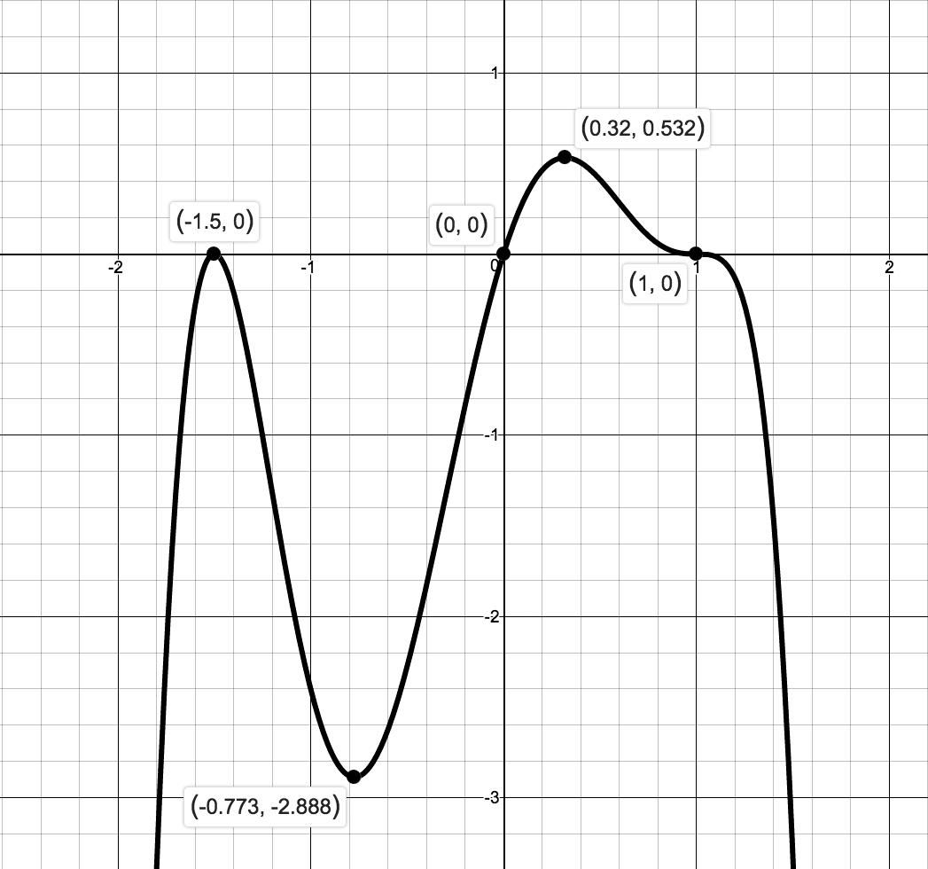
Below is a graph of a polynomial function \(y = p(x)\) as generated by a graphing utility. Answer the following questions about \(p\) based
on the graph provided.
List the real zeros of \(p\) along with their respective multiplicities.
The zeros appear to be: \(x=-1.5\), even multiplicity - probably \(2\) since it doesn’t ‘look like’ the graph is very flat near \(x = 2\); \(x=0\), odd
multiplicity - probably \(1\) since the graph seems fairly linear as it passes through the origin; \(x=1\) odd multiplicity - probably \(3\) or
higher since the graph seems fairly ‘flat’ near \(x = 1\).
List the local minimums and local maximums of the graph of \(y = p(x)\).
local minimum: approximately \((-0.773, -2.888)\); local maximums: approximately \((-1.5,0)\), and \((0.32, 0.532)\)
What can be said about the degree of and leading coefficient \(p(x)\)?
Based on the graph, even degree (at least \(6\) based on multiplicities) with a negative leading coefficient based on the
end behavior.
It turns out that \(p(x)\) is a seventh degree polynomial. (to be exact, \(p(x) = -0.1\left (x+1.5\right )^2\left (3x\right )\left (x-1\right )^3\left (x+5\right )\).) How can this be?
We only have a portion of the graph represented here.
(This Exercise is a follow up to Example graphfromtheory.) Use a graphing utility to compare and contrast the graphs of \(f(x) = (2x-1)(x+1)^2(1-x)(x^2+1)\) and \(g(x) = (2x-1)(x+1)^2(1-x)\).
Use the graph of \(y= p(x) = (2x-1)(x+1)(1-x^4)\) (the graph which directly precedes Example boxnotopex) to estimate the largest open interval containing \(x = -0.235\) which
satisfies the the criteria for ‘local minimum’ in Definition localmaxmindefn.
We are looking for the largest open interval containing \(x = -0.235\) for which the graph of \(y = p(x)\) is at or above \(y=-1.121\). Since each of the gridlines on
the \(x\)-axis correspond to \(0.2\) units, we approximate this interval as \((-1.25 \, \text {ish}, 1.1 \, \text {ish})\).
In light of Definition localmaxmindefn, explain why every point on the graph of a constant function is both a local maximum and a local
minimum.
This exercise involves the greatest integer function, \(f(x) = \lfloor x \rfloor \), introduced in Example greatestintegerdefn. Explain why the points \((k,k)\) for integers \(k\) are local
maximums but not local minimums.
Here are a few other questions for you to discuss with your classmates.
How many and how few local extrema could a polynomial of degree \(n\) have?
Could a polynomial have two local maxima but no local minima?
If a polynomial has two local maxima and two local minima, can it be of odd degree? Can it be of even degree?
Can a polynomial have local extrema without having any real zeros?
Why must every polynomial of odd degree have at least one real zero?
Can a polynomial have two distinct real zeros and no local extrema?
Can an \(x\)-intercept yield a local extrema? Can it yield an absolute extrema?
If the \(y\)-intercept yields an absolute minimum, what can we say about the degree of the polynomial and the sign
of the leading coefficient?
(This is a follow-up to Exercises LagrangeLinearExercise in Section LinearFunctions and LagrangeQuadExercise in Section QuadraticFunctions.) The Lagrange Interpolate function \(L\) for four points: \((x_{0}, y_{0})\), \((x_{1}, y_{1})\), \((x_{2}, y_{2})\), \((x_{3}, y_{3})\) where \(x_{0}\),
\(x_{1}\), \(x_{2}\), and \(x_{3}\) are four distinct real numbers is given by the formula:
Choose four points with different \(x\)-values and construct the Lagrange Interpolate for those points. Verify each
of the points lies on the polynomial.
Verify that, in general, \(L(x_{0}) = y_{0}\), \(L(x_{1}) = y_{1}\), \(L(x_{2}) = y_{2}\), and \(L(x_{3}) = y_{3}\).
Find \(L(x)\) for the points \((-1,1)\), \((0,0)\), \((1,1)\) and \((2,4)\). What happens?
\(L(x) = x^2\)
Find \(L(x)\) for the points \((-1,0)\), \((0,1)\), \((1,2)\) and \((2,3)\). What happens?
\(L(x) = x+1\)
Generalize the formula for \(L(x)\) to five points. What’s the pattern?
 PreCalculus
![[Picture]](ExercisesforGraphsofPolynomials.online-af6aec2e6463172dd523401857078827.svg)
![[Picture]](ExercisesforGraphsofPolynomials.online-8dbc7a30f61e08f8998430190814f1b2.svg)
![[Picture]](ExercisesforGraphsofPolynomials.online-d8d25ac6688275761578b0a60a782b7b.svg)
![[Picture]](ExercisesforGraphsofPolynomials.online-dbd4ca2f90147dab31c04331f2cee8b9.svg)
![[Picture]](ExercisesforGraphsofPolynomials.online-39808a1f121fdf12d6441358c15a9fbe.svg)